
Master Excel PivotTables: Summarize Data with Ease
Learn to create, customize, and analyze data with Excel PivotTables in simple, step-by-step instructions. Discover how to prepare your data, use the PivotTable Fields pane, and apply interactive filters like slicers for instant insights. Gain control over large datasets and generate clear reports effortlessly.
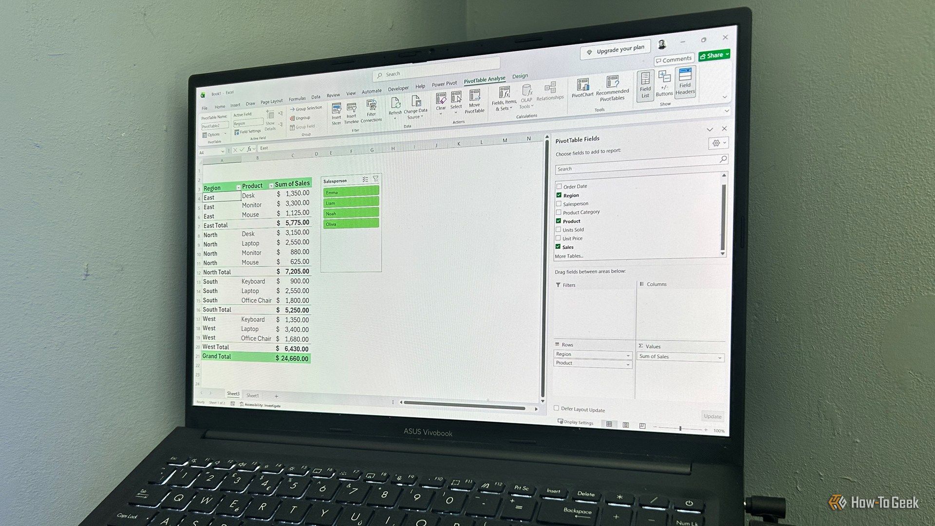
Microsoft Excel PivotTables may seem complex, but they are powerful, drag-and-drop tools that can transform thousands of rows of raw data into clear, meaningful reports in minutes. This guide will walk you through the essential steps to create, customize, and analyze your data using PivotTables, all without altering your original spreadsheet. You'll learn how to prepare your data, build your first PivotTable, understand its core components, and use interactive features like slicers to gain insights instantly.
Prepare Your Data for Success
Accurate and well-structured source data is the foundation of any reliable PivotTable. Before you begin, ensure your data follows these best practices:
- Unique Headers: Every column in your dataset must have a unique, descriptive header. These headers become the fields you use in your PivotTable.
- No Blank Rows: Avoid leaving any entirely blank rows within your dataset. These can confuse Excel and prevent it from accurately recognizing your data range.
- Consistent Formatting: Ensure dates are formatted as dates and numbers are formatted as numbers. Inconsistent formatting can lead to incorrect calculations or unexpected grouping in your PivotTable.
- Convert to an Excel Table: Select any cell in your data range and press Ctrl+T, or go to Insert > Table. Converting your raw data into an official Excel Table is a vital step because tables automatically expand when you add new rows. This means your PivotTable will include any new data simply by refreshing it, saving you the effort of rebuilding your layout.
Following these steps ensures your data is clean and ready for powerful analysis.
Create Your First PivotTable
Once your data is properly structured, creating a PivotTable is straightforward:
- Select a Cell: Click on any single cell within your Excel Table. This tells Excel which data to use.
- Insert PivotTable: Go to the Insert tab on the Excel ribbon, then click the top half of the PivotTable button.
- Choose Location: In the 'Create PivotTable' dialog box, you'll be asked where to place the new PivotTable. For better organization and to keep your raw data separate from your analysis, it's generally recommended to select New Worksheet.
- Confirm: Click OK. Excel will open a new worksheet with a blank PivotTable area and display the 'PivotTable Fields' pane on the right side of your screen.
Understand the PivotTable Fields Pane
Your new PivotTable will initially appear blank, waiting for you to define what data you want to summarize. The 'PivotTable Fields' pane is your control center. It lists all the column headers from your source data (these are your 'fields') at the top, and four crucial report areas below:
- Rows: Fields dragged here will display their unique categories down the left side of your report.
- Columns: Fields placed here will display their unique categories across the top of your report.
- Values: This is where Excel performs calculations on your data. Numeric fields are typically summed by default, while text fields are counted. This area provides the core quantitative summary of your report.
- Filters: Dragging a field here adds an interactive filter menu above your PivotTable, allowing you to quickly isolate the entire report based on specific criteria (e.g., viewing sales for a particular region).
You can interact with this pane in two ways: either check the box next to a field name and let Excel automatically place it in an appropriate area, or drag and drop fields directly into the desired report area. As you add or rearrange fields, your PivotTable will update instantly. Remember, your source data remains untouched, so feel free to experiment with different arrangements until your PivotTable tells the story you need.
Troubleshooting Tip: If the 'PivotTable Fields' pane disappears, simply click anywhere inside your PivotTable, then navigate to the PivotTable Analyze tab (which appears contextually on the ribbon) and click Field List.
Best Practice: Customizing Value Calculations
You aren't limited to just summing values. You can drag the same numeric field (e.g., "Sales") into the Values area multiple times. To change the calculation for a duplicate field:
- Click the drop-down arrow next to the duplicated field in the Values area (e.g., "Sum of Sales2").
- Select Value Field Settings.
- Choose a different summary function such as Count, Average, Max, or Min.
To remove a field, click its drop-down arrow in one of the report areas and select Remove Field, or simply drag it out of the area.
Master the PivotTable Analyze Tab
When you select a cell within your PivotTable, a contextual PivotTable Analyze tab appears on your Excel ribbon. This tab provides essential tools for managing and enhancing your PivotTable, including data refreshing and interactive filtering.
Refreshing Your Data
If you make changes to your original source data (the Excel Table), your PivotTable won't update automatically. You need to refresh it:
- Click the Refresh button in the PivotTable Analyze tab, or press Alt+F5.
- If your workbook contains multiple PivotTables or external data connections, expand the Refresh drop-down menu and choose Refresh All to update everything at once.
Adding Interactive Slicers
Slicers provide a highly visual and interactive way to filter your PivotTable data. Instead of using the small filter buttons within the PivotTable, slicers offer a panel of buttons you can click to instantly filter your report by specific categories.
To insert a slicer:
- With your PivotTable selected, go to the PivotTable Analyze tab.
- Click Insert Slicer.
- In the 'Insert Slicers' dialog, check the box next to the column(s) you want to use as a filter (e.g., "Salesperson" or "Product").
- Click OK. Excel will place an interactive button panel on your sheet. You can then click these buttons to dynamically filter your PivotTable data.
Conclusion and Next Steps
You've now learned the fundamental steps to create and use PivotTables in Excel. By preparing your data, understanding the PivotTable Fields pane, and utilizing the tools in the PivotTable Analyze tab, you can quickly summarize, analyze, and gain valuable insights from large datasets. Continue experimenting with different field arrangements and summary calculations to unlock the full potential of PivotTables.
To further enhance your data analysis skills, explore creating PivotCharts for visual representation of your PivotTable data, or delve into more advanced PivotTable features like calculated fields and grouping.
FAQ
Q: Why is my PivotTable completely blank after creation?
A: A blank PivotTable means you haven't yet told Excel what data to summarize. You need to drag fields from the 'PivotTable Fields' list into the Rows, Columns, and Values areas of the pane. For example, drag 'Region' to Rows and 'Sales' to Values to see total sales by region.
Q: How do I change the calculation for a value field, like from Sum to Average?
A: In the 'PivotTable Fields' pane, locate the field you want to change in the 'Values' area. Click the drop-down arrow next to its name (e.g., "Sum of Sales"), then select Value Field Settings. From there, you can choose a different summary function like Count, Average, Max, or Min.
Q: I added new rows to my source data, but my PivotTable isn't showing them. What should I do?
A: Your PivotTable needs to be refreshed to include new data. First, ensure your source data is formatted as an Excel Table (this allows it to automatically expand to include new rows). Then, click anywhere in your PivotTable, go to the PivotTable Analyze tab, and click the Refresh button. If you have multiple PivotTables, select Refresh All from the drop-down menu.
Related articles

TCG Pocket Responds: A Much-Needed Pace Shift for Pokémon Fans
Pokémon TCG Pocket is rolling out a major update for its second anniversary, primarily addressing player concerns about overwhelming content releases by shifting to a six-week set schedule. This aims to curb player decline and improve overall engagement by giving trainers more time to collect and strategize. The update also adds new collection methods, improved deck-building features, and enhanced trading functionality.
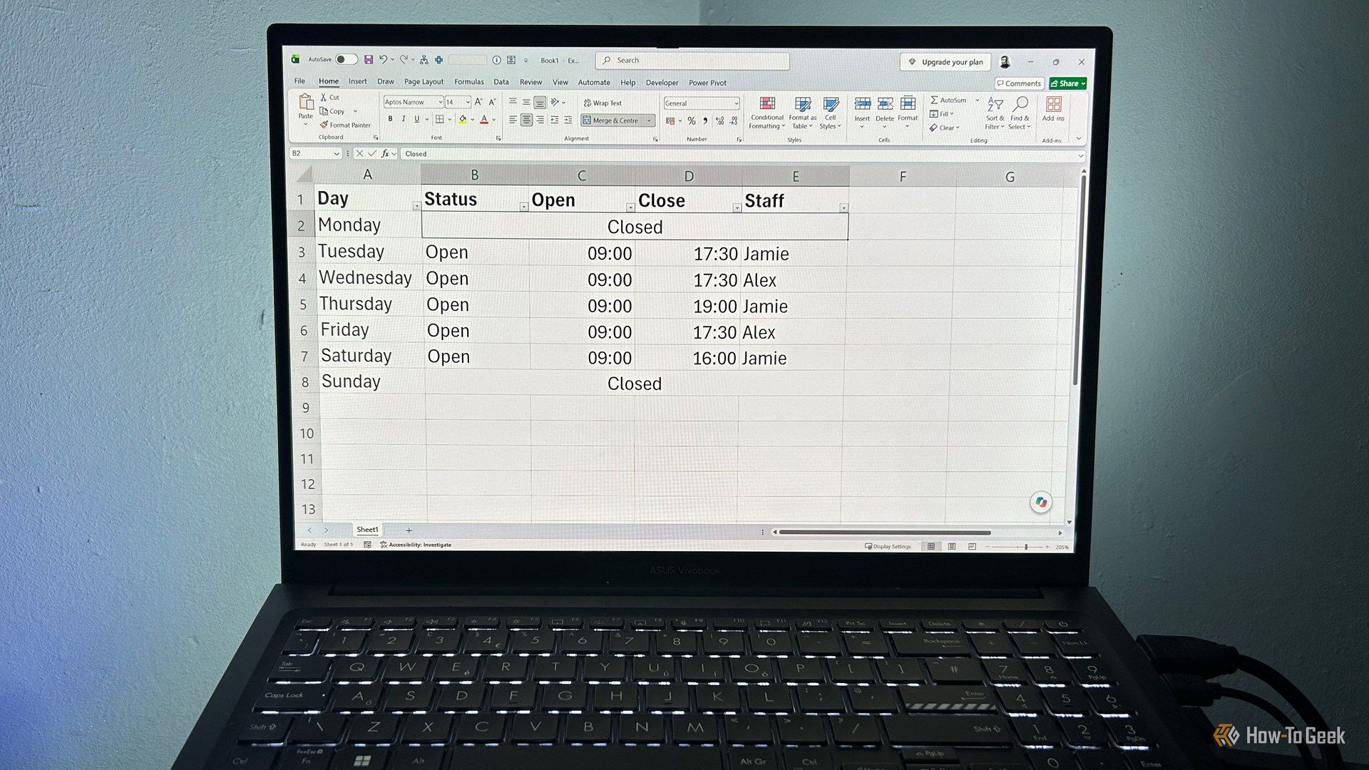
Ditch Merge & Center: The Better Way to Align Text in Excel
Learn to use Excel's "Center Across Selection" to align text across cells without merging, avoiding common data manipulation issues. This guide provides steps to utilize this newly accessible feature and add it to your Quick Access Toolbar.

AI's Confidence vs. Formal Methods' Rigor: Design Flaws & Verification
While AI accelerates code generation, formal methods remain critical for ensuring system correctness. Languages like TLA+ and tools like Quint enable developers to model and verify system designs before coding, catching subtle flaws. Quint makes formal methods more accessible with developer-friendly syntax and executability. This approach is vital for verifying AI-generated code through trace validation and model-based testing, ensuring reliability against real-world data.
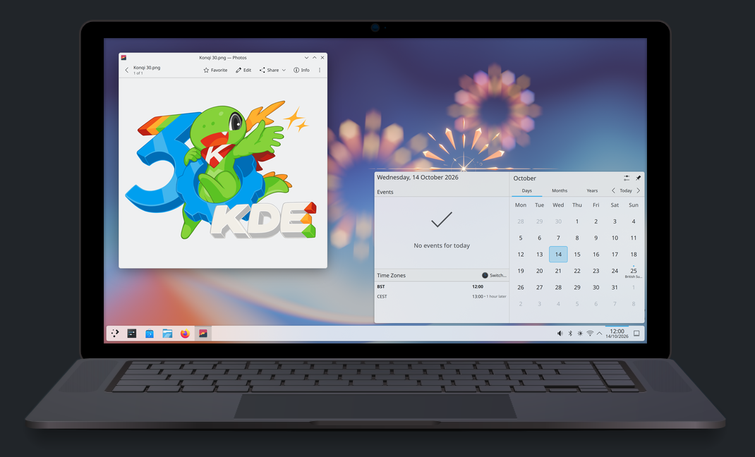
KDE Plasma 6.8: A Future-Focused 30th Anniversary Update
Quick Verdict KDE Plasma 6.8, arriving as the "30th Anniversary Edition," is a pivotal release that decisively pushes the desktop environment into the future. With a definitive farewell to native X11 sessions and a

regional: A two-person Seattle startup lands $1M to reinvent
Seattle startup TriMagnetix has secured $1 million to develop semiconductor chips that consume 800 times less energy and are radiation-resistant. The two-person company, leveraging nanomagnetic technology, is targeting space applications and data centers. With new funding and key partnerships, TriMagnetix aims for commercial sales within a year.

Ephemeral PR Preview Environments on GKE: A Deep Dive
Every development team eventually grapples with the limitations of shared staging environments. The familiar scenario: multiple features deployed simultaneously, database migrations clashing, and the phrase "it works on