
Analyzing Analyst Estimate Ranges with Python for Deeper Insights
Most financial models rely on a single consensus estimate for forward-looking inputs like revenue or EPS. While convenient, this approach flattens crucial data, reducing complex expectations to just an average. The

Most financial models rely on a single consensus estimate for forward-looking inputs like revenue or EPS. While convenient, this approach flattens crucial data, reducing complex expectations to just an average. The reality is that behind every average estimate, there's a range – a low estimate, a high estimate, and a count of analysts contributing. Two companies might share the same average estimate, but the level of agreement (or disagreement) among analysts could be vastly different. This article explores how to move beyond a single number and use Python to analyze the shape of analyst consensus, revealing where true uncertainty lies.
Why Go Beyond the Average?
Consider two companies: one with a revenue estimate of $100 million, where all analysts predict between $99M and $101M, and another with the same $100M average, but estimates ranging from $80M to $120M. A model treating both as simply '$100M' misses the significant difference in underlying analyst confidence. By analyzing the low, average, and high estimates, alongside the number of analysts, we can uncover patterns of consensus disagreement, guiding more informed financial modeling.
Setting Up Your Environment and Data Acquisition
To follow along, you'll need Python 3.9+ and familiarity with pandas DataFrames, basic plotting, and financial concepts like revenue and EPS. Ensure you have an FMP API key and the following libraries installed:
python import requests import pandas as pd import numpy as np import matplotlib.pyplot as plt from datetime import datetime from time import sleep
Our goal is to fetch annual analyst estimates including low, average, high, and analyst counts for both revenue and EPS across a diverse set of tickers. This mixed universe helps prevent biased results that might arise from focusing solely on heavily covered mega-cap stocks.
Here’s how to pull the data for a predefined list of tickers, ensuring we select the nearest usable future estimate period:
python api_key = 'YOUR FMP API KEY' base_url = 'https://financialmodelingprep.com/stable' tickers = [ 'AAPL', 'MSFT', 'NVDA', 'AMZN', 'META', 'GOOGL', 'TSLA', 'PLTR', 'COIN', 'RBLX', 'SNOW', 'UBER', 'AMD', 'INTC', 'MU', 'AVGO', 'QCOM', 'CAT', 'DE', 'BA', 'GE', 'XOM', 'CVX', 'WMT', 'COST', 'NKE', 'SBUX', 'MCD', 'TGT', 'JPM', 'BAC', 'GS', 'MS', 'V', 'MA', 'UNH', 'PFE', 'LLY', 'MRK', 'ABBV', 'ROKU', 'SHOP', 'SQ', 'PYPL', 'ZM' ]
all_rows = [] today = pd.Timestamp.today().normalize() for ticker in tickers: url = f'{base_url}/analyst-estimates' params = { 'symbol': ticker, 'period': 'annual', 'limit': 10, 'apikey': api_key } response = requests.get(url, params=params) data = response.json() df = pd.DataFrame(data) if len(df) == 0: print(f'{ticker}: no data') continue df['date'] = pd.to_datetime(df['date']) df = df.sort_values('date') df = df[ (df['date'] > today) & (df['revenueAvg'].notna()) & (df['revenueLow'].notna()) & (df['revenueHigh'].notna()) & (df['epsAvg'].notna()) & (df['epsLow'].notna()) & (df['epsHigh'].notna()) ].copy() if len(df) == 0: print(f'{ticker}: no usable future estimates') continue row = df.iloc[0].copy() all_rows.append(row) print(f'{ticker} done') sleep(0.2) estimates = pd.DataFrame(all_rows)
This script fetches the necessary granular data, providing a foundational DataFrame with the average estimate, its range, and the analyst count for each company.
Quantifying Uncertainty: From Raw Ranges to Spread Metrics
Raw estimate ranges are not directly comparable across companies of varying sizes. A $10 billion revenue range means something very different for a $50 billion company than for a $500 billion one. To normalize this, we calculate a spread metric by dividing the difference between high and low estimates by the average estimate.
python estimates['revenue_spread'] = ((estimates['revenueHigh'] - estimates['revenueLow']) / estimates['revenueAvg']) estimates['eps_spread'] = ((estimates['epsHigh'] - estimates['epsLow']) / estimates['epsAvg'].abs()) shape_df = estimates[['symbol','date','revenueLow','revenueAvg','revenueHigh','revenue_spread','numAnalystsRevenue', 'epsLow','epsAvg','epsHigh','eps_spread','numAnalystsEps']].copy()
For EPS spread, an important consideration is when the average EPS is close to zero. In such cases, even a small absolute range can result in a disproportionately large percentage spread, which might not accurately reflect true uncertainty. To mitigate this, we create a clean_eps_spread column, flagging or setting to NaN values where the absolute average EPS is very low or the spread is excessively high.
python shape_df['eps_spread_clean'] = shape_df['eps_spread'] shape_df.loc[shape_df['epsAvg'].abs() < 1, 'eps_spread_clean'] = np.nan shape_df.loc[shape_df['eps_spread_clean'] > 3, 'eps_spread_clean'] = np.nan
By sorting companies based on these spread metrics, we can immediately see where analyst agreement is tightest or widest. For instance, some companies might show wide revenue estimate ranges despite significant analyst coverage, while others might have a tight revenue spread but a much wider EPS spread, signaling that disagreement sits specifically around profitability.
Visualizing Consensus Dynamics
To better understand the relationship between analyst coverage and estimate uncertainty, we can plot these metrics. A straightforward approach involves categorizing companies based on median thresholds for analyst count and revenue spread.
We define four basic consensus shapes for revenue:
- Tight Consensus: High analyst coverage, low revenue spread.
- Watched but Uncertain: High analyst coverage, high revenue spread.
- Thin but Stable: Low analyst coverage, low revenue spread.
- Weak Consensus: Low analyst coverage, high revenue spread.
Plotting the number of analysts against the revenue estimate spread clearly illustrates that extensive coverage doesn't automatically translate to tight agreement. Companies like MSFT and AAPL might show tight consensus, but others like TSLA or NVDA, despite high coverage, can exhibit wide revenue estimate spreads, falling into the 'watched but uncertain' category.
However, a more insightful view emerges when we compare revenue uncertainty with EPS uncertainty. This helps pinpoint whether the disagreement is about top-line growth, profitability, or both.
By establishing median thresholds for both revenue_spread and eps_spread_clean, we can categorize companies into four distinct forecast shapes:
- Stable Forecast Shape: Low revenue uncertainty and low EPS uncertainty (e.g., MSFT).
- Profitability Uncertainty: Low revenue uncertainty but high EPS uncertainty (e.g., SQ, SNOW, PLTR).
- Top-Line Uncertainty: High revenue uncertainty but low EPS uncertainty (a smaller group).
- Broad Forecast Uncertainty: High revenue uncertainty and high EPS uncertainty (e.g., TSLA).
This classification provides a richer context than a single average estimate. For example, Square (SQ) might show a very tight revenue spread (around 1%), but a significantly wide EPS spread (over 70%). This indicates that analysts largely agree on revenue generation but diverge considerably on the company's profitability or earnings conversion. Conversely, a company like Tesla (TSLA) often exhibits broad forecast uncertainty, with wide spreads in both revenue and EPS, signaling disagreement across multiple model components.
Practical Takeaways for Your Forecasting Workflow
The key insight is not to discard analyst estimates, but to enrich them. Instead of just storing estimated_revenue and estimated_eps, consider expanding your data model to include:
symbol | estimated_revenue | estimated_eps | revenue_spread | eps_spread | analyst_count | forecast_shape
Integrating these additional metrics provides crucial context, allowing your models to understand the confidence (or lack thereof) behind each input. It helps differentiate between a tightly clustered consensus and one with significant internal disagreement, even if their averages are identical. This allows for more nuanced scenario analysis and risk assessment within your financial forecasting.
Important Considerations and Limitations
It's vital to remember that this analysis uses simplified median thresholds for categorization and a handpicked universe of stocks for illustrative purposes. It's not a formal statistical model or a predictive tool for stock returns. The primary goal is to reveal the structure of consensus, not to determine the correctness of any specific estimate. Always exercise caution when interpreting EPS spreads, especially for companies with EPS values close to zero, as these can easily distort the percentage spread. This method is about understanding the landscape of analyst opinion, not predicting the future.
FAQ
Q: Why is it necessary to clean the eps_spread?
A: When the average EPS (the denominator) is very close to zero, even a small absolute difference between the high and low estimates can result in an extremely large and potentially misleading percentage spread. Cleaning the eps_spread by setting it to NaN for near-zero average EPS or capping excessively high values prevents these outliers from distorting the analysis and visualizations.
Q: How does a "watched but uncertain" company differ from a "weak consensus" company?
A: A "watched but uncertain" company has high analyst coverage (many analysts following it) but still exhibits a wide estimate spread. This suggests widespread disagreement despite significant attention. In contrast, a "weak consensus" company has both low analyst coverage and a wide estimate spread, indicating disagreement compounded by a shallower analyst bench.
Q: Can this approach predict which estimates are more likely to be accurate?
A: No, this analysis is not designed to predict the accuracy of analyst estimates. Its purpose is purely descriptive: to uncover the underlying structure and level of agreement or disagreement within the consensus. A tight consensus doesn't guarantee accuracy, nor does a wide spread necessarily mean the estimate is wrong; it merely indicates differing opinions among analysts.
Related articles

AI's Confidence vs. Formal Methods' Rigor: Design Flaws & Verification
While AI accelerates code generation, formal methods remain critical for ensuring system correctness. Languages like TLA+ and tools like Quint enable developers to model and verify system designs before coding, catching subtle flaws. Quint makes formal methods more accessible with developer-friendly syntax and executability. This approach is vital for verifying AI-generated code through trace validation and model-based testing, ensuring reliability against real-world data.
Ephemeral PR Preview Environments on GKE: A Deep Dive
Every development team eventually grapples with the limitations of shared staging environments. The familiar scenario: multiple features deployed simultaneously, database migrations clashing, and the phrase "it works on
Secure Internal API Access for AI Agents with MCP
AI agents accessing internal APIs directly pose significant risks, including identity loss, unrestricted queries, and security bypasses. The Model Context Protocol (MCP) offers a solution by defining explicit tools. A secure architecture involves an MCP server wrapping the API with strict input validation, coupled with a gateway that handles authentication, rate limiting, and audit logging, ensuring safe and accountable access.
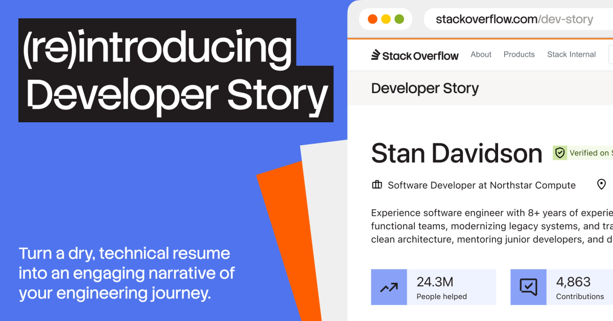
Beyond the Resume Noise: Developer Story Rethinks Tech Hiring
Stack Overflow is addressing the growing challenges in tech hiring, exacerbated by AI's influence leading to untrustworthy and generic resumes. Their solution, the re-introduced Developer Story, offers a platform for developers to authentically showcase their work, expertise, and impact through verifiable contributions and personal projects. This aims to provide hiring teams with more objective insights and help genuine talent stand out in a crowded market.
Adding & Validating JSON-LD Structured Data in Next.js
When we build websites, we want them to be discoverable and accurately understood by search engines. This isn't just about keywords and meta descriptions anymore; it's about providing explicit, machine-readable context.

Build Scalable AI Automations with n8n for Production Workflows
As software developers, we're constantly pushing the boundaries of what automation can achieve. While connecting a couple of applications with basic triggers is straightforward, constructing AI-powered workflows that